xspec Documentation¶

Download this notebook.

This ipython Notebook is intended to provide documentation for the linetools GUI named XSpecGUI.

Enjoy and feel free to suggest edits/additions, etc.

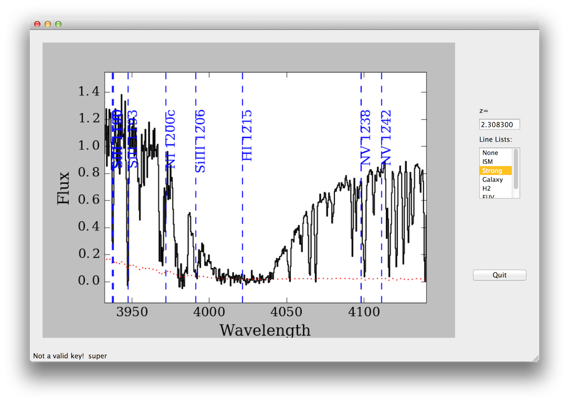
Here is a screenshot of the XSpecGUI in action:

from IPython.display import Image
Image(filename="images/xspec_example.png")

The example spectrum file used below is part of the linetools package.

import imp
lt_path = imp.find_module('linetools')[1]
spec_fil = lt_path+'/spectra/tests/files/PH957_f.fits'

Before Launching the GUI¶

If you are a Mac user, we highly recommend that you set your matplotlib backend from MacOSX to TkAgg (or another option, see backends).

Launching the GUI¶

From the command line (recommended)¶

We recommend you use the script provided with linetools.

Then it is as simple as:

> lt_xspec filename

Here are the current command-line options:

> lt_xspec -h
usage: lt_xspec [-h] [--zsys ZSYS] [--norm] [--exten EXTEN]
                [--wave_tag WAVE_TAG] [--flux_tag FLUX_TAG]
                [--sig_tag SIG_TAG] [--var_tag VAR_TAG] [--ivar_tag IVAR_TAG]
                file

Parse for XSpec

positional arguments:
  file                 Spectral file

optional arguments:
  -h, --help           show this help message and exit
  --zsys ZSYS          System Redshift
  --norm               Show spectrum continuum normalized (if continuum is
                       provided)
  --exten EXTEN        FITS extension
  --wave_tag WAVE_TAG  Tag for wave in Table
  --flux_tag FLUX_TAG  Tag for flux in Table
  --sig_tag SIG_TAG    Tag for sig in Table
  --var_tag VAR_TAG    Tag for var in Table
  --ivar_tag IVAR_TAG  Tag for ivar in Table

From within ipython or equivalent¶

from linetools.guis import xspecgui as ltxsg

import imp; imp.reload(ltxsg)
ltxsg.main(spec_fil)

Navigating - These key strokes help you explore the spectrum (be sure to click in the spectrum panel first!)¶

Setting the window edges (mouse+keystroke)¶

l – Set left edge of window
r – Set right edge of window
t – Set top edge of window
b – Set bottom edge of window
Z – Set bottom edge to 0.
W – View full spectrum
s,s – Set a zoom-in window at 2 mouse positions

Zoom in/out Wavelength¶

i – Zoom in on cursor
I – Zoom in extra fast
o – Zoom out
O – Zoom out extra fast

Best estimate Flux limits¶

y – Make a guess for the flux plotting limits

Zoom out Flux¶

Y – Zoom out

Pan¶

[ – Pan left
{ – Pan left extra
] – Pan right
} – Pan right extra

Overlaying Line Lists¶

You can overlay a series of vertical lines at standard spectral lines at any given redshift.

Setting the Line List¶

You must choose a line-list by clicking one.

Setting the redshift¶

Type one in
RMB on a spectral feature (Ctrl-click on Emulated 3-button on Macs)
- Choose the rest wavelength

Marking Doublets¶

C – CIV
M – MgII
X – OVI
4 – SiIV
8 – NeVIII
B – Lyb/Lya

Velocity plot (Coming Soon)¶

Once a line list and redshift are set, type ‘v’ to launch a Velocity Plot GUI.

Simple Analysis¶

Gaussian Fit¶

You can fit a Gaussian to any single feature in the spectrum as follows: 1. Click “G” at the continuum at one edge of the feature 1. And then another “G” at the other edge (also at the continuum) 1. A simple Gaussian is fit and reported.

Equivalent Width¶

You can measure the rest EW of a spectral feature as follows: 1. Click “E” at the continuum at one edge of the feature 1. And then another “E” at the other edge (also at the continuum) 1. A simple boxcar integration is performed and reported.

Apparent Column Density¶

You can measure the apparent column via AODM as follows: 1. Click “N” at the continuum at one edge of the feature 1. And then another “EN” at the other edge (also at the continuum) 1. A simple AODM integration is performed and reported.

Ly\(\alpha\) Lines¶

“D” - Plot a DLA with \(N_{\rm HI} = 10^{20.3} \rm cm^{-2}\)
“R” - Plot a SLLS with \(N_{\rm HI} = 10^{19} \rm cm^{-2}\)

Table Of Contents